HOOPS AI Inside a HOOPS Visualize Desktop + Exchange Application: Similar-Part Search Across 10,000 CAD Files
Last time I confirmed that a native application can call HOOPS AI directly through a C ABI bridge with CPython embedded in it (Using HOOPS AI from a Fully Local Desktop Application). That client was a console app, though, so the results came back as numbers and labels and nothing more. This time I dropped the same bridge into a desktop application built on HOOPS Visualize Desktop and HOOPS Exchange, and built a sample that can run MFR (manufacturing feature recognition) and similar-part search on the 3D CAD models it imports.
Everything I set out to do works. Per-face feature recognition shows up as colors in the view; two parts can be compared as an AI similarity score and a geometric diff at the same time; roughly 10,000 CAD files go into an index that you browse as a thumbnail list and query for similar parts; and the clusters you find can be tagged and then viewed as a whole in a Shape Embedding Map. All of it inside a single desktop application.

That is what the application looks like. The view is showing the Shape Embedding Map described below — how close the registered parts sit to one another, as a point cloud, with the legend on the left and the Similarity Search panel on the right. The UI is an ordinary HOOPS Visualize Desktop application, and nothing about it hints that Python is running underneath.
The thing I was least sure about going in was how a desktop application would cope with an index of that size. Behind FastAPI or MCP you can hand the heavy work to a server and wait for it asynchronously. In a native app, a call into the bridge blocks right there, and in the end it is the GUI thread that has to render 10,000 entries. Whether that holds up in practice was the main thing I wanted to find out.
Approach
The starting point was qt_sandbox, the Qt sample application that ships with HOOPS Visualize Desktop. I added exactly two things to its UI: a “HOOPS AI” menu (MFR Inference, Similarity Comparison, Similarity Search) and a Similarity Search dock panel on the right. Everything on the AI side is handled by the bridge from the previous article (hoops_ai_native_bridge). The bridge ships as an include/lib/bin package, the same layout as the HOOPS SDKs, so wiring it into the project is no different from adding any other HOOPS SDK. What actually took the effort, though, wasn’t calling the C ABI — it was building an application that can handle 10,000 files. More on that below.
One addition on the CAD side: to use A3DCompareFacesInBrepModels for Similarity Comparison, the application also calls the raw HOOPS Exchange C API (A3D API) directly. qt_sandbox has a USING_EXCHANGE preprocessor definition that turns on Exchange Sprocket file I/O, which is how the CAD files handed to HOOPS AI are opened, so all of the new code lives inside that definition.
I picked qt_sandbox out of all the samples because the same project builds and runs on Linux. Having made the bridge work on both Windows and Linux, it would defeat the point to put it in an application that only runs on one of them. The screenshots here are from Windows, but I have built the same source tree with qmake on an Ubuntu 24.04 desktop and run MFR and similar-part search there as well. And if HOOPS AI supports macOS one day, a Qt-based application should not be hard to move over.
What I found
The tutorial workflow reproduces in a native application

The first milestone was getting out of Jupyter. You can try every HOOPS AI feature in the tutorial notebooks, but that isn’t the same as being able to put them in a product. The question was whether a workflow that runs in a notebook also runs inside an ordinary desktop application.
MFR was the first thing I checked. Pick MFR Inference from the “HOOPS AI” menu and every face of the loaded model is colored by its recognized feature, with a legend in the upper right. circular_end_pocket, blind_hole, through_hole, fillet and the rest are listed there along with how many faces each one accounts for. The same results the notebook produces, from a single menu item.
Initialization and loading the .ckpt happen exactly once. A trained model stays resident for the lifetime of the process, so there is nothing to wait for on the second inference and every one after it. For a desktop application that cost cannot be paid per call, so it was one of the first things I wanted to confirm.
Adding AI to an application that already exists

Load two parts, run Similarity Comparison, and two results come back at once. One is a per-face diff from HOOPS Exchange’s
A3DCompareFacesInBrepModels, which colors the view by faces that match, faces only in the old model, and faces only in the new one. The other is a cosine similarity from HOOPS AI’s shape embeddings, shown just below the legend.
AI is being layered onto applications of every kind right now, and 3D applications won’t be an exception. This is one small example of what that looks like. Shape comparison is an existing feature; put a machine-learned similarity score next to the color-coded result and the impact of a design change — the thing an experienced engineer used to size up by eye — becomes a number.
A 10,000-file index stays responsive

Point the Similarity Search panel at a folder and everything under it goes into the index, listed with thumbnails. Turn search on and the parts most similar to the currently open model are ranked by score, with a slider at the top to move the threshold and narrow the list on the spot.
The data set here is roughly 10,000 CAD files, and they aren’t all single parts: about 8,400 are, and the other 2,400-odd are assemblies, which comes to just over 42,000 bodies in total.
Above is a search for an F2B two-bolt flange bearing unit with a grease nipple. Eleven other units with a nipple follow, down to 0.9623, and then the score drops to 0.9014 at the point where the ones without it begin. It’s a tiny protrusion relative to the whole part, but the embedding picks the difference up and it shows in the ranking.
The concern I opened with turned out to be unfounded: with roughly 10,000 files in the index, neither scrolling the list nor dragging the threshold ever stuttered. That doesn’t come for free, though. Build the list as a naive QListWidget and 10,000 items will bring it to its knees. This application uses model/view virtualization, asynchronous thumbnail decoding with a cache, and a debounce on the threshold slider.
And the work wasn’t confined to the client side. Once the list is virtualized, there is no point receiving the contents of the index all at once — you need to be able to ask for just the range you are about to show. So I added HoopsAI_ListIndexPartsPaged to the bridge, which takes an offset and a count. Building the bridge first and putting an application on top of it isn’t a one-way street; what the application needs pushes back on the bridge’s design.
Identical results to the tutorial, and faster
Part search runs in two stages. First the embedding retrieves candidates from FAISS; then CADSearch’s geometric reranker rescores them using shape measures such as the oriented bounding box. The score you see in the gallery is a blend of the two. The bridge runs the same implementation the tutorial does (run_part_search → search_by_shape), unchanged.


Query the same index with the same bevel gear and the hits, the scores and the ranking all come back identical. The time taken did differ, though: 3.8 seconds on the qt_sandbox side including the overhead of the bridge call, against 12.3 seconds for the same work in the notebook. Most of that gap is presumably Jupyter’s own overhead. A notebook is a fine place to check that a feature does what you expect; as the UI of something people use daily, it’s a different game.
Indexing got faster and failures dropped by more than 10x
So how did those 10,000 files get into the index? A trained model is something you can prepare elsewhere and bring in, but registering shapes for similar-part search is work that happens continuously — so that belongs in the application. Parts can be added one at a time, or a whole folder can be registered at once.
I started by running the same 10,000 files through the tutorial notebook: 270 of them failed to register, most of those on timeouts. The bridge at that point was just the tutorial’s sample code wrapped behind a C ABI, so calling it from the application gave me no way to do anything about that.

So I exposed
num_workers and the time limit through the bridge and split the job in two: Pass 1 runs every file in parallel, and Pass 2 picks up the heavy files that fell out of it with fewer workers and a much longer limit.
Those four values are seeded from the machine they run on, but they are editable. Core count, free memory and how heavy the data is all differ from one environment to the next, so the defaults are a starting point you can move from.
embed_shape_batch also has parameters of its own for this — per-size-bucket time limits, and a policy for what to do with files flagged as too heavy — and tuning those is another way to go (Embed_shape_batch() Specifications Guide). I wanted a comparison against the tutorial, though, so I kept the call itself on the same terms and put Pass 2 in the application instead.
Here is what registering 10,897 files looked like, next to the same data set run through the Jupyter notebook tutorial. Pass 1 uses the same worker count and time limit as the tutorial.
| Workers | Time limit | Elapsed | Files processed | Failures | |
|---|---|---|---|---|---|
| Jupyter notebook tutorial | 12 | 120 s (default) | 228 min 36 s | 10,897 | 270 |
| qt_sandbox / Pass 1 | 12 | 120 s | 184 min 06 s | 10,897 | 186 |
| qt_sandbox / Pass 2 | 4 | 1200 s | 172 min 01 s | 186 | 22 |
| qt_sandbox / total | — | — | 356 min 07 s | 10,897 | 22 |
Pass 1 is supposed to be an apples-to-apples run, and yet it finishes 44 minutes sooner than the tutorial and fails on 84 fewer files. I don’t have an explanation for that. The work being called and the degree of parallelism are the same, so I suspect overhead from going through Jupyter, but I haven’t confirmed it. The part search above showed a gap in the same direction. Whatever the cause, if you are shipping HOOPS AI to end users, it looks like the thing to do is get it out of Jupyter and run it as plain Python — through the bridge, in this case.
Pass 2 then recovers 164 of those 186 failures, bringing the final count down to 22, or 0.20%. The total time is longer, but that extra time is spent deliberately on the heavy files that would otherwise have been dropped.
The remaining 22 are not a matter of allowing more time. Fourteen fail immediately with deterministic CAD errors. The other eight either never return from the native side or take the worker process down with them. I confirmed they still don’t finish with the limit raised to 1800 seconds before reporting them, along with a related issue: when a worker dies, the supervisor doesn’t notice and waits out the full time limit anyway. Both have since been addressed and are due in the next release.
From tagging to the Shape Embedding Map, the whole unsupervised workflow

When similar-part search turns up a coherent group, you can tag it. In the example above, Bevel Gears, Spur Gears, Bushings, Crankshafts, Corner brackets, Support brackets and the rest are clusters I found by searching and named afterwards — 20 of them, as the legend shows. Tags are written as JSON next to the index, so they survive closing the application.
Open the Shape Embedding Map from there and the tagged parts are collected and drawn as a point cloud in the view. The embeddings have 2048 dimensions and can’t be plotted as they are, so principal component analysis picks the three directions that best account for how the parts differ from each other, and the points are projected onto those three axes. Each point takes the color of its tag, with a legend in the upper left. The panel list narrows to the tagged parts at the same time, so the map and the list are always showing the same set.
Worth noting: positions on this map come purely from proximity in the embedding space — none of the geometric rescoring that shapes part search is involved. Search is there to rank precisely what is closest to one part; the map is there to show you the distribution as a whole.
Flattening 2048 dimensions into three has obvious limits, and in a still image the depth collapses too, so the GIF above rotates the view. Watching it turn, Bevel Gears and Spur Gears blend together near the center, and the grease nipple that cost those search hits a few points shows up as two adjacent clusters — the groupings a person would call “the same kind of thing” are reflected in the embedding space reasonably well.
The whole flow feels a lot like Google Photos: keep adding pictures and the same face gets grouped on its own, and then you’re asked who that person is. Here you drop in 10,000 unlabeled CAD files, parts with similar shapes gather into clusters, and you get to say “these are the bevel gears.” Confirming that a workflow we take for granted with photographs also holds for 3D shapes, with my own hands and with HOOPS AI, was the part I enjoyed most.
For real use, being able to search by shape is valuable in itself. Part numbering schemes and part names differ from one division to the next, but geometry is common ground — which makes it possible to catch the duplicate design that gets created because nobody knew a similar part already existed, and from there to standardize and reduce the part count. And when a similar part from the past comes back, so does everything recorded against it: material, heat treatment, tolerances, surface finish.
HOOPS AI doesn’t stop at looking things up, either. With the Context Layer, the metadata that the retrieved parts carry in PLM or ERP can be used to predict what’s missing for the part in hand — material, manufacturing process, routing, cost. Predictions come with a confidence and fall into three buckets: ready to propose as is, needs a human review, or not enough evidence to predict at all. It is an attempt to reproduce, starting from geometry alone, the call an experienced engineer would make at a glance at the drawing. This sample application doesn’t go that far, but a production system probably would.
Copy the folder and it runs on another Windows machine
The last thing I wanted to check was whether this application can be shipped. HOOPS AI’s site-packages is too large to carry wholesale, so the bridge comes with a procedure that runs the features you actually use, pulls just the modules that got imported out of site-packages, and collects them along with the build output and the checkpoints into a single package. The Qt application drops straight into that same framework.
<package>\
├── bin\                       exe and every DLL (Qt / Visualize / Exchange / bridge)
├── .venv\
│   └── Lib\site-packages\     HOOPS AI (narrowed down by the trace)
├── models\                    *.ckpt
├── materials\                 from Visualize\samples\data\materials
├── fonts\                     from Visualize\fonts
└── resource\                  from Exchange\bin\resource
The key point is that no environment variables are required. If HVISUALIZE_INSTALL_DIR and the rest are set, the application still looks at the development tree as before; if they aren’t, it assumes the package layout above and resolves everything relative to the exe.
I tested this on a freshly launched Windows Server instance on AWS. Copying the package over and starting it from a remote desktop session was enough: MFR, similar-part search, and parallel indexing of a whole folder all worked. No installer, no launcher.
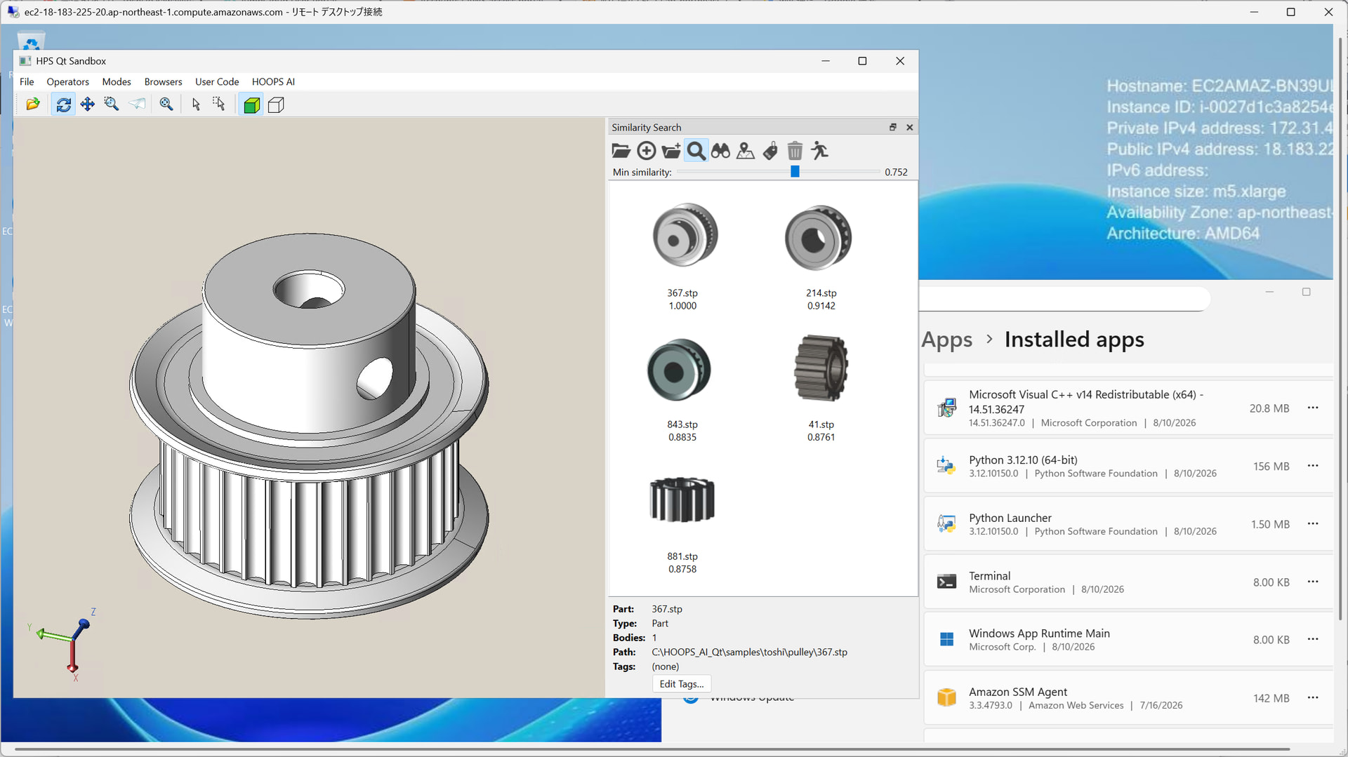
It isn’t a completely bare machine, to be clear. As the installed apps list behind the window shows, Python 3.12 (the python.org installer) and the Visual C++ redistributable (x64) do have to be there. Then again, that is all that has to be there.
So the path an ISV partner would take to ship this inside their own product and hand it to end users is connected end to end. What you are allowed to include, though, is a separate question from what technically runs. Whether HOOPS AI itself and the trained checkpoints can be redistributed — and equally the HOOPS Visualize Desktop and HOOPS Exchange binaries in the package — depends on the terms of the Technology Partner Agreement (TPA) and varies by country and by agreement.
The package also contains Qt DLLs, and those have nothing to do with your agreement with Tech Soft 3D: they follow Qt’s own licensing, LGPL or commercial. What you ship comes from different places under different terms, and no single agreement covers all of it. That is why the bridge’s packaging step emits a manifest that separates what came from Tech Soft 3D from what came from third parties — so the sorting is done up front. Either way, please don’t take this post as the answer; check the terms that apply to you.
Three consumers of Exchange in one process, and it just works
One more thing worth writing down, about Exchange. In this application there are three of them in the same process: the Exchange that HOOPS Visualize Desktop (HPS) uses to import CAD into the scene graph, the raw A3D API the application calls itself, and the Exchange that HOOPS AI uses internally. They coexist without any special handling.
Each holds its own function pointer table, so as bindings they don’t interfere with each other. The physical DLL, however, is one module shared at the OS level, and the Tf* kernel underneath collapses into a single instance. Which means all three have to be on the same version of Exchange. Here, HOOPS Visualize Desktop and HOOPS Exchange are both 2026.2.0 to match HOOPS AI V1.1. Obvious once stated, but a mismatch here produces crashes that are hard to trace back, so it is worth settling the combination first.
Verdict
Everything I wanted to check came back as “it works.” The tutorial workflow reproduces on the desktop side, initialization and the .ckpt load happen once per session, an index of 10,000 files registers, lists and searches at practical speed, and the flow from tagging through to the Shape Embedding Map runs end to end. On top of that, the application can be copied as a folder onto a machine with neither HOOPS AI nor the HOOPS SDKs installed and still run.
That said, none of it happens simply because you call the bridge. Handling 10,000 files takes UI virtualization and asynchronous thumbnails, and it took adding a paging function to the bridge to support them. The worker count and time limits for bulk registration only settle after you try a few values on the machine you’re on. Integrating it is no different from any other HOOPS SDK; standing up to data at real scale takes a fair amount of work on top.
There is homework left. Both trained models here — MFR and similar-part search — are the .ckpt files that come with the tutorials. In production you would build models against your own industry’s parts and your own label scheme, which brings the training phase into the picture. Everything above ran on CPU, which is fine for inference, but training needs a GPU. Covering training from a native application would mean adding GPU support, in the bridge as well.
A note: this is a PoC, not a product
To be clear, this application exists to find out whether HOOPS AI can be made to work inside a native app. It is not something you would ship as is.
The trained-model question above is the clearest illustration. What this sample is really meant to show is the vessel those models go into. The SDK combination, moving CAD data around, registering data at volume, the UI work — all of that is needed regardless of which model you use. Get through it once and adapting it to your own domain becomes a matter of swapping the model.
Source
The full sample application is at toshi-bata/hoops_ai_qt_sandbox. Build steps, the SDK versions you need, and the environment variables are in the README, so cloning it and following along should get you the same thing on your own machine. The bridge it calls into is at toshi-bata/hoops_ai_native_bridge. As always, treat this as a starting point rather than production-quality code.
One thing to note: you need a unified key with HOOPS AI, HOOPS Visualize Desktop and HOOPS Exchange all enabled (a single key covers all three). HOOPS AI is available for evaluation, so with a key that includes the three you can run the whole workflow described here against your own CAD data. Please give it a try.
What’s next
Getting to the settings behind that two-pass registration took a series of overnight benchmark runs. How I swept num_workers and the time limits, and why those particular values, is a post of its own — I’ll write it up separately.
Questions, comments, or results from your own data — happy to hear them in this thread.